2: Basic contrasts (single stratum) • ratesci

library(ratesci)

Confidence intervals for comparisons of independent binomial or Poisson rates

SCAS and other asymptotic score methods

For comparison of two groups when the outcome is a binomial proportion, you may wish to quantify the effect size using the difference ( $\hat \theta_{RD} = \hat p_1 - \hat p_2$ , where $\hat p_i = x_i/n_i$ ) or the ratio of the two proportions ( $\hat \theta_{RR} = \hat p_1 / \hat p_2$ ). Another option is the odds ratio ( $\hat \theta_{OR} = \hat p_1 (1 - \hat p_2) / \hat p_2(1 - \hat p_1)$ ), which is less easy to interpret, but is widely used due to its useful properties for logistic regression modelling or case-control studies.

To calculate a confidence interval (CI) for any of these contrasts, the skewness-corrected asymptotic score (SCAS) method is recommended, as one that succeeds, on average, at containing the true parameter $\theta$ with the appropriate nominal probability (e.g. 95%), and has evenly distributed tail probabilities (Laud 2017). It is a modified version of the Miettinen-Nurminen (MN) asymptotic score method (Miettinen and Nurminen 1985). MN and SCAS each represent a family of methods encompassing analysis of RD and RR for binomial proportions or Poisson rates (e.g. exposure-adjusted incidence rate), and binomial OR.

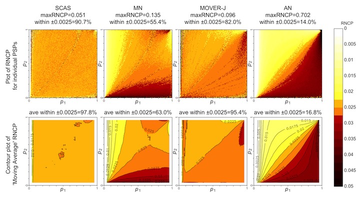
The plots below illustrate the one-sided and two-sided interval coverage probabilities¹ achieved by SCAS compared to some other popular methods² with $(n_1, n_2) = (45, 15)$ , with the second row of each plot using moving average smoothing. A selection of coverage probability plots for other sample size combinations and other contrasts can be found in the “plots” folder of the ratesci GitHub repository.

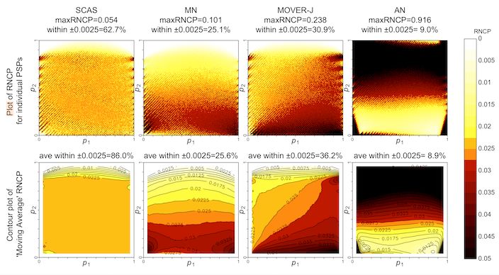
Differences in two-sided coverage can be more subtle:

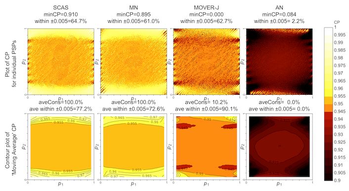
The skewness correction, introduced by (Gart and Nam 1988) should be considered essential for analysis of relative risk, but can also have a substantial effect for RD as seen above. The one-sided coverage of MN for RR can be poor even in large samples with equal-sized groups, which means that the confidence interval tends to be located too close to 1:

[Note: (Morten W. Fagerland, Lydersen, and Laake 2011) dismissed the MN method, saying that it can be somewhat liberal. In fact, based on reconstruction of their results, it appears that their evaluation was of the closely-related but inferior Mee method, which omits the N/(N-1) variance bias correction. This error was corrected in their 2017 book. Essentially, it seems they reject the MN method on the basis of some very small regions of the parameter space where coverage is slightly below nominal. These dips in coverage do occur, but fluctuate above and below the nominal level in a pattern of ridges and furrows aligned along the diagonal of a fixed value of $\theta_{RD}$ . The most severe dips tend to occur when sample sizes are multiples of 10 (e.g. $(n_1, n_2) = (40, 10)$ ), which might be relatively rare in practice. The moving average smoothing in the above surface plots is designed to even out these fluctuations in coverage. The ‘N-1’ adjustment in the MN method elevates coverage probabilities slightly, and the skewness correction gives a further improvement overall, as well as substantially improving one-sided coverage when group sizes are unequal.]

scoreci() is used as follows, for example to obtain a SCAS 95% CI for the difference 5/56 - 0/29:

out <- scoreci(x1 = 5, n1 = 56, x2 = 0, n = 29)
out$estimates
#>        lower    est upper level x1 n1 x2 n2  p1hat p2hat  p1mle p2mle
#> [1,] -0.0186 0.0917 0.187  0.95  5 56  0 29 0.0893     0 0.0917     0

The underlying z-statistic is used to obtain a two-sided hypothesis test for association (pval2sided). Note that under certain conditions (i.e. $n_1 = n_2$ ) this is equivalent to the Egon Pearson ‘N-1’ chi-squared test (Campbell 2007). The facility is also provided for a custom one-sided test against any specified null hypothesis value $\theta_0$ , e.g. for non-inferiority testing (pval_left and pval_right). See the tests vignette for more details.

out$pval
#>      chisq pval2sided theta0 scorenull pval_left pval_right
#> [1,]  3.02      0.082      0      1.74     0.959      0.041

The scoreci() function provides options to omit the skewness correction (skew = FALSE for the MN method) and the variance bias correction (bcf = FALSE for the Mee method, which would be consistent with the Karl Pearson unadjusted chi-squared test). To keep things simple when choosing the SCAS method, you may instead use the scasci() wrapper function instead of scoreci():

scasci(x1 = 5, n1 = 56, x2 = 0, n = 29)$estimates
#>        lower    est upper level x1 n1 x2 n2  p1hat p2hat  p1mle p2mle
#> [1,] -0.0186 0.0917 0.187  0.95  5 56  0 29 0.0893     0 0.0917     0

For analysis of relative risk, use:

scasci(x1 = 5, n1 = 56, x2 = 0, n = 29, contrast = "RR")$estimates
#>      lower  est upper level x1 n1 x2 n2  p1hat p2hat  p1mle  p2mle
#> [1,]  0.77 16.4   Inf  0.95  5 56  0 29 0.0893     0 0.0868 0.0053

And for odds ratio:

scasci(x1 = 5, n1 = 56, x2 = 0, n = 29, contrast = "OR")$estimates
#>      lower  est upper level x1 n1 x2 n2  p1hat p2hat  p1mle   p2mle
#> [1,] 0.759 17.7   Inf  0.95  5 56  0 29 0.0893     0 0.0865 0.00533

For analysis of Poisson incidence rates, for example exposure-adjusted adverse event rates, the same methodology is adapted for the Poisson distribution, with the distrib argument. So, for example if the denominators 56 and 29 represent the number of patient-years at risk in each group, instead of the number of patients:

scasci(x1 = 5, n1 = 56, x2 = 0, n = 29, contrast = "RR", distrib = "poi")$estimates
#>      lower  est upper level x1 n1 x2 n2  p1hat p2hat  p1mle   p2mle
#> [1,] 0.726 16.1   Inf  0.95  5 56  0 29 0.0893     0 0.0865 0.00539

MOVER methods

An alternative family of methods to produce confidence intervals for the same set of binomial and Poisson contrasts is the Method of Variance Estimates Recovery (MOVER), also known as Square-and-Add (For technical details see chapter 7 of Newcombe 2012). Originally labelled as a “Score” method (Newcombe 1998) due to the involvement of the Wilson Score interval, this involves a combination of intervals calculated separately for $p_1$ and $p_2$ . Newcombe based his method on Wilson intervals, but coverage can be slightly improved by using equal-tailed Jeffreys intervals instead (“MOVER-J”) (Laud 2017)³. Coverage properties remain generally inferior to SCAS - with larger sample sizes, MOVER-J has two-sided coverage close to (but slightly below) the nominal level, but central location is not achieved (except for the RR contrast).

There is no corresponding hypothesis test for the MOVER methods.

A MOVER-J interval for binomial RD from the same observed data as above would be obtained using:

moverci(x1 = 5, n1 = 56, x2 = 0, n = 29)
#> $estimates
#>         lower   est upper level x1 n1 x2 n2  p1hat   p2hat
#> [1,] -0.00973 0.084 0.177  0.95  5 56  0 29 0.0918 0.00775
#> 
#> $call
#>  distrib contrast    level     type      adj       cc       a1       b1 
#>    "bin"     "RD"   "0.95"   "jeff"  "FALSE"  "FALSE"    "0.5"    "0.5" 
#>       a2       b2 
#>    "0.5"    "0.5"

For comparison, Newcombe’s version using Wilson intervals is:

moverci(x1 = 5, n1 = 56, x2 = 0, n = 29, type = "wilson")
#> $estimates
#>        lower    est upper level x1 n1 x2 n2  p1hat p2hat
#> [1,] -0.0381 0.0893 0.193  0.95  5 56  0 29 0.0893     0
#> 
#> $call
#>  distrib contrast    level     type      adj       cc       a1       b1 
#>    "bin"     "RD"   "0.95" "wilson"  "FALSE"  "FALSE"    "0.5"    "0.5" 
#>       a2       b2 
#>    "0.5"    "0.5"

The MOVER approach may be further modified by adapting the Jeffreys interval (which uses a non-informative $Beta(0.5, 0.5)$ prior for the group rates) to incorporate prior information about $p_1$ and $p_2$ for an approximate Bayesian interval. For example, given data from a pilot study with 1/10 events in the first group and 0/10 in the second group, the non-informative $Beta(0.5, 0.5)$ prior distributions for $p_1$ and $p_2$ might be updated as follows:

moverbci(x1 = 5, n1 = 56, x2 = 0, n = 29, a1 = 1.5, b1 = 9.5, a2 = 0.5, b2 = 10.5)
#> $estimates
#>        lower    est upper level x1 n1 x2 n2 p1hat   p2hat
#> [1,] 0.00917 0.0872 0.172  0.95  5 56  0 29 0.093 0.00578
#> 
#> $call
#>  distrib contrast    level     type      adj       cc       a1       b1 
#>    "bin"     "RD"   "0.95"   "jeff"  "FALSE"      "0"    "1.5"    "9.5" 
#>       a2       b2 
#>    "0.5"   "10.5"

WARNING: Note that confidence intervals for ratio measures should be equivariant, in the sense that:

interchanging the groups produces reciprocal intervals for RR or OR, i.e. the lower and upper confidence limits for $x_1/n_1$ vs $x_2/n_2$ are the reciprocal of the upper and lower limits for $x_2/n_2$ vs $x_1/n_1$
in addition for OR, interchanging events and non-events produces reciprocal intervals, i.e. the lower and upper confidence limits for the odds ratio of $(n_1 - x_1)/n_1$ vs $(n_2 - x_2)/n_2$ are the reciprocal of the upper and lower limits for $x_1/n_1$ vs $x_2/n_2$ .

Unfortunately, the MOVER method for contrast = “OR”, as described in (Morten W. Fagerland and Newcombe 2012), does not satisfy the second of these requirements.

Technical details

(Miettinen and Nurminen 1985) took the concept of the Wilson score interval for a single proportion and applied it to all contrasts of two proportions (not just RD) and Poisson rates. The procedure involves finding, at any possible value of the contrast parameter $\theta$ , the maximum likelihood estimates of the two proportions, restricted to the given value of $\theta$ . The resulting estimates are then included in the score statistic, and the confidence interval found by an iterative root-finding algorithm. Miettinen and Nurminen’s statistic was defined to follow a $\chi^2_1$ distribution, but the SCAS formula uses an equivalent statistic with a N(0, 1) distribution, to facilitate one-sided tests.

Gart and Nam, in a series of papers between 1985 and 1990, proposed similar confidence interval methods that included a skewness correction in the score statistic (and also a bias correction for OR). Their formulae omitted the ‘N-1’ bias correction used by Miettinen and Nurminen.

Farrington and Manning published an article on non-inferiority tests for RD and RR, using the same restricted maximum likelihood methodology as Miettinen and Nurminen (but omitting the ‘N-1’ correction).

The SCAS method combines the features of all the above methods, to give a comprehensive family of asymptotic score methods with optimised performance for universal use for confidence intervals for a wide range of sample sizes, with coherent tests for association or for non-inferiority. For further details, see (Laud 2017).

References

Campbell, Ian. 2007. “Chi-Squared and FisherIrwin Tests of Two-by-Two Tables with Small Sample Recommendations.” Statistics in Medicine 26 (19): 3661–75. https://doi.org/10.1002/sim.2832.

Fagerland, Morten W, Stian Lydersen, and Petter Laake. 2011. “Recommended Confidence Intervals for Two Independent Binomial Proportions.” Statistical Methods in Medical Research 24 (2): 224–54. https://doi.org/10.1177/0962280211415469.

Fagerland, Morten W., and Robert G. Newcombe. 2012. “Confidence Intervals for Odds Ratio and Relative Risk Based on the Inverse Hyperbolic Sine Transformation.” Statistics in Medicine 32 (16): 2823–36. https://doi.org/10.1002/sim.5714.

Gart, John J., and Jun-mo Nam. 1988. “Approximate Interval Estimation of the Ratio of Binomial Parameters: A Review and Corrections for Skewness.” Biometrics 44 (2): 323. https://doi.org/10.2307/2531848.

Laud, Peter J. 2017. “Equal-Tailed Confidence Intervals for Comparison of Rates.” Pharmaceutical Statistics 16 (5): 334–48. https://doi.org/10.1002/pst.1813.

Miettinen, Olli, and Markku Nurminen. 1985. “Comparative Analysis of Two Rates.” Statistics in Medicine 4 (2): 213–26. https://doi.org/10.1002/sim.4780040211.

Newcombe, Robert G. 1998. “Interval Estimation for the Difference Between Independent Proportions: Comparison of Eleven Methods.” Statistics in Medicine 17 (8): 873–90. https://doi.org/10.1002/(sici)1097-0258(19980430)17:8<873::aid-sim779>3.0.co;2-i.

———. 2012. Confidence Intervals for Proportions and Related Measures of Effect Size. CRC Press. https://doi.org/10.1201/b12670.