4: Paired contrasts • ratesci

library(ratesci)

Confidence intervals and tests for paired comparisons of binomial proportions

The input data for paired proportions takes a different structure, compared with the data for independent proportions:

		Event B
		Success	Failure	Total
Event A	Success	$a \ (p_{11})$	$b \ (p_{12})$	$x_1 = a + b \ (p_1)$
	Failure	$c \ (p_{21})$	$d \ (p_{22})$	$c + d \ (1 -p_1)$
	Total	$x_2 = a + c \ (p_2)$	$b + d \ (1 - p_2)$	$N$

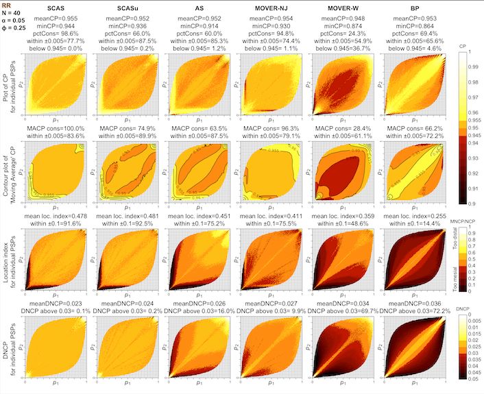
SCAS and other asymptotic score methods for RD and RR

To calculate a confidence interval (CI) for a paired risk difference ( $\hat{\theta}_{RD} = \hat{p}_1 - \hat{p}_2$ , where $\hat{p}_1 = (a+b)/N$ , $\hat{p}_2 = (a+c)/N$ ), or relative risk ( $\hat{\theta}_{RR} = \hat{p}_1 / \hat{p}_2$ ), the skewness-corrected asymptotic score (SCAS) method is recommended, as one that succeeds, on average, at containing the true parameter $\theta$ with the appropriate nominal probability (e.g. 95%), and has evenly distributed tail probabilities (Laud 2026, under review). It is a modified version of the asymptotic score methods by (Tango 1998) for RD, and (Nam and Blackwelder 2002) and (Tang et al. 2003) for RR, incorporating both a skewness correction and a correction in the variance estimate.

The plots below illustrate the one-sided and two-sided interval coverage probabilities achieved by SCAS compared to some other popular methods¹, when $N=40$ and the correlation coefficient is 0.25. A selection of coverage probability plots for other sample sizes and correlations can be found in the “plots” folder of the cpplot GitHub repository.

scorepairci() takes input in the form of a vector of length 4, comprising the four values c(a, b, c, d) from the above table, which are the number of paired observations having each of the four possible pairs of outcomes.

For example, using the dataset from a study of airway reactivity in children before and after stem cell transplantation, as used in (Fagerland et al. 2014):

out <- scorepairci(x = c(1, 1, 7, 12), precis = 4)
out$estimates
#>        lower     est   upper level  p1hat p2hat  p1mle  p2mle phi_hat phi_c
#> [1,] -0.5281 -0.2859 -0.0184  0.95 0.0952 0.381 0.0952 0.3811  0.0795     0
#>      psi_hat
#> [1,]  1.7143

The underlying z-statistic is used to obtain a two-sided hypothesis test against the null hypothesis of no difference (pval2sided). Note that this is equivalent to an ‘N-1’ adjusted version of the McNemar test. The facility is also provided for a custom one-sided test against any specified null hypothesis value $\theta_0$ , e.g. for non-inferiority testing (pval_left and pval_right). See the tests vignette for more details.

out$pval
#>         chisq pval2sided theta0 scorenull  pval_left pval_right
#> [1,] 4.285714 0.03843393      0 -2.070197 0.01921697   0.980783

For a confidence interval for paired RR, use:

out <- scorepairci(x = c(1, 1, 7, 12), contrast = "RR", precis = 4)
out$estimates
#>       lower    est  upper level  p1hat p2hat  p1mle  p2mle phi_hat phi_c
#> [1,] 0.0429 0.2627 0.9282  0.95 0.0952 0.381 0.0994 0.3785  0.0795     0
#>      psi_hat
#> [1,]  1.7143
out$pval
#>         chisq pval2sided theta0 scorenull  pval_left pval_right
#> [1,] 4.285714 0.03843393      1 -2.070197 0.01921697   0.980783

To obtain the legacy Tango and Tang intervals for RD and RR respectively, you may set the skew and bcf arguments to FALSE. Also switching to closedform = TRUE takes advantage of closed-form calculations for these methods (whereas the SCAS method is solved by iteration).

MOVER methods

For application of the MOVER method to paired RD or RR, an estimate of the correlation coefficient is included in the formula. A correction to the correlation estimate, introduced by Newcombe, is recommended, obtained with corc = TRUE. As for unpaired MOVER methods, the default base method used for the individual (marginal) proportions is the equal-tailed Jeffreys interval, rather than the Wilson Score interval as originally proposed by Newcombe (obtained using type = "wilson"). The combination of the Newcombe correlation estimate and the Jeffreys intervals gives the designation “MOVER-NJ”. This method is less computationally intensive than SCAS, but coverage properties are inferior, and there is no corresponding hypothesis test.

moverpairci(x = c(1, 1, 7, 12), contrast = "RD", corc = TRUE, precis = 4)$estimates
#>        lower     est   upper level  p1hat p2hat phi_hat
#> [1,] -0.5105 -0.2857 -0.0324  0.95 0.0952 0.381       0

For cross-checking against published example in (Fagerland et al. 2014)

moverpairci(x = c(1, 1, 7, 12), contrast = "RD", corc = TRUE, type = "wilson", precis = 4)$estimates
#>        lower     est   upper level  p1hat p2hat phi_hat
#> [1,] -0.5069 -0.2857 -0.0256  0.95 0.0952 0.381       0

Conditional odds ratio

Confidence intervals for paired odds ratio are obtained conditional on the number of discordant pairs, by transforming a confidence interval for the proportion $b / (b+c)$ . Transformed SCAS (with or without a variance bias correction, to ensure consistency with the above SCAS hypothesis tests for RD and RR) or transformed mid-p intervals are recommended (Laud 2026, under review).

out <- scorepairci(x = c(1, 1, 7, 12), contrast = "OR")
out$estimates
#>         lower      est    upper
#> [1,] 0.007702 0.161863 0.912316
out$pval
#>         chisq pval2sided theta0 scorenull  pval_left pval_right
#> [1,] 4.285714 0.03843393      1 -2.070197 0.01921697   0.980783

To select an alternative method, for example transformed mid-p:

orpairci(x = c(1, 1, 7, 12))$estimates
#>                           lower       est     upper
#> Transformed SCASp    0.00770217 0.1428571 0.9123154
#> Transformed midp     0.00629101 0.1428571 0.9241027
#> Transformed Wilson   0.02293156 0.1428571 0.8899597
#> Transformed Jeffreys 0.01403242 0.1428571 0.8305608
#> Wald                 0.01757637 0.1428571 1.1611135

References

Fagerland, Morten W., Stian Lydersen, and Petter Laake. 2014. “Recommended Tests and Confidence Intervals for Paired Binomial Proportions.” Statistics in Medicine 33 (16): 2850–75. https://doi.org/10.1002/sim.6148.

Nam, Jun-mo, and William C. Blackwelder. 2002. “Analysis of the Ratio of Marginal Probabilities in a Matched-Pair Setting.” Statistics in Medicine 21 (5): 689–99. https://doi.org/10.1002/sim.1017.

Tang, Nian-Sheng, Man-Lai Tang, and Ivan Siu Fung Chan. 2003. “On Tests of Equivalence via Non-Unity Relative Risk for Matched-Pair Design.” Statistics in Medicine 22 (8): 1217–33. https://doi.org/10.1002/sim.1213.

Tango, Toshiro. 1998. “Equivalence Test and Confidence Interval for the Difference in Proportions for the Paired-Sample Design.” Statistics in Medicine 17 (8): 891–908. https://doi.org/10.1002/(sici)1097-0258(19980430)17:8<891::aid-sim780>3.0.co;2-b.